Training Guide

This section goes over the most important metrics and settings to achieve a balanced generator/discriminator adversarial training, where both models converge and learn from each other.

Best Practices

It is recommended to use the training warmups and schedulers as explained above. The following images present how these practices are reflected in the logs.

Objectives and loss composition

The generator and discriminator are optimised with a weighted sum of reconstruction, perceptual, and adversarial criteria so you can balance spectral fidelity against perceptual sharpness: $$ \mathcal{L}{\text{total}} = \lambda}} \mathcal{L{\text{L1}} + \lambda}} \mathcal{L{\text{perc}} + \lambda}} \mathcal{L{\text{adv}} + \lambda}} \mathcal{L{\text{SAM}} + \lambda. $$ Each coefficient maps directly to the }} \mathcal{L}_{\text{TV}Training.Losses block in the configuration file, mirroring the weighted-sum description from the paper. Typical setups emphasise pixel/L1 and perceptual terms early on, then ramp in adversarial weight to sharpen textures once the discriminator has warmed up.

Exponential Moving Average (EMA)

For smoother validation curves and more stable inference, the trainer can maintain an exponential moving average of the generator parameters. After each optimisation step, the EMA weights (\theta_{\text{EMA}}) are updated toward the current generator state (\theta): $$ \theta_{\text{EMA}}^{(t)} = \beta \, \theta_{\text{EMA}}^{(t-1)} + (1 - \beta)\, \theta^{(t)}, $$ where the decay (\beta \in [0,1)) controls how much history is retained. During validation and inference, the EMA snapshot replaces the live weights so that predictions are less sensitive to short-term oscillations. The final super-resolved output therefore comes from the smoothed generator, $$ \hat{y}{\text{SR}} = G(x; \theta), $$ which empirically reduces adversarial artefacts and improves perceptual consistency.}

Generator LR Warmup

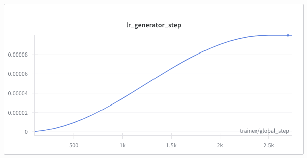
When starting to train, the learning rate slowly rises from 0 to the indicated value. This prevents exploding gradients after random initialization of the weights when training the model from scratch. The length of the LR warmup is defined with the Schedulers.g_warmup_steps parameter in the config. Whether the increase is linear or smoother is defined with the Schedulers.g_warmup_type setting; ideally this should be set to cosine.

Generator Pre-training

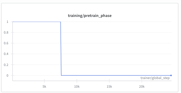
After the loss stabilizes, the generator continues to be trained while the discriminator sits idle. This prevents the discriminator from overpowering the generator in early training stages, where the generator output is still easily identifiable as synthetic. The binary flag training/pretrain_phase is logged to indicate whether the model is still in pretraining. Whether pretraining is enabled is defined with the Training.pretrain_g_only parameter in the config; Training.g_pretrain_steps defines how many steps this pretraining takes in total. The parameter Training.g_warmup_steps defines how many training steps (batches) the smooth LR increase lasts; setting it to 0 turns it off.

During this generator-only pretraining window, the optimization target is hardwired to plain L1 loss only. Once pretraining ends, the normal configured content-loss mix (L1/SAM/perceptual/TV) is used again.

Discriminator

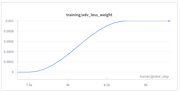
Once the training/pretrain_phase flag is 0, pretraining of the generator is no longer active and the discriminator starts to be trained. Not only is it trained, but its true/false prediction is also added to the generator to start the adversarial game. To avoid training the generator on low-quality discriminator outputs at this early stage, we gradually feed the discriminator output to the generator as a loss. For that, we slowly increase the adversarial loss weight from 0 to the predetermined amount. The loss weight is logged to WandB in order to visualize the influence this loss has on the generator.

Continued Training

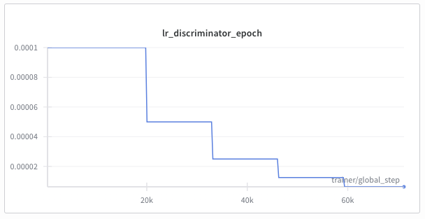
As training continues, the generator tries to fool the discriminator, while the discriminator tries to distinguish between real and synthetic samples. We monitor the overall loss of both models independently. When the overall loss metric of one model reaches a plateau, we reduce its learning rate to train the model optimally. . The patience, LR decrease factor in case of a plateau, and the metric used for these LR schedulers are all defined individually for (G) and (D) in the Schedulers section of the config file.

The schedulers now expose a cooldown period and min_lr floor. Cooldown waits a configurable number of epochs before watching for the next plateau, preventing back-to-back reductions, while min_lr guarantees that the optimiser never stalls at zero. Use these knobs to keep the momentum of long trainings without overshooting into vanishing updates.

TTUR, Adam defaults and gradient clipping

Both optimisers use a two-time-scale update rule (TTUR) so the discriminator defaults to a slower learning rate than the generator. The bundled Adam configuration mirrors popular GAN recipes with betas set to (0.0, 0.99) and eps=1e-7, ensuring the generator reacts quickly to discriminator feedback without building up stale momentum. Weight decay is automatically restricted to convolutional and dense kernels—normalisation layers and biases are excluded—so regularisation never interferes with running statistics. Finally, gradient_clip_val applies global norm clipping when set above zero; values between 0.5 and 1.0 work well when discriminator spikes cause unstable updates.

ESRGAN checkerboard mitigation (10m defaults)

If you observe faint checkerboard textures, especially in flat/low-frequency areas, start with: - Generator.use_icnr: True to initialise PixelShuffle pre-convolutions with ICNR. - Optimizers.optim_d_lr <= 0.5 * optim_g_lr to keep discriminator pressure in check. - Training.Losses.fixed_idx: [0, 1, 2] for 4-band inputs so VGG perceptual loss uses RGB consistently.

Final stages of the Training

With further progression of training, it is important not only to monitor the absolute reconstruction quality of the generator, but also to keep an eye on the balance between the generator and discriminator. Ideally, we try to reach the Nash equilibrium, where the discriminator cannot distinguish between real and synthetic anymore, meaning the super-resolution is (at least for the discriminator) indistinguishable from the real high-resolution image. This equilibrium is achieved when both (D(y)) and (D(G(x))) approach 0.5.

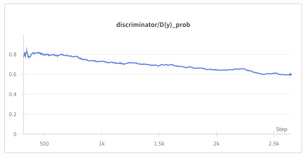
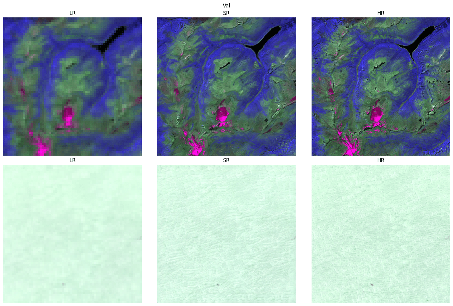
Also keep an eye out on the example images that are logged at every validation step. .